
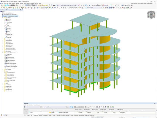
The building model is calculated in two phases:
- Global 3D calculation of the global model, where the slabs are modeled as a rigid plane (diaphragm) or as a bending plate
- Local 2D calculation of the individual floors
After the calculation, the results of the columns and walls from the 3D calculation and the results of the slabs from the 2D calculation are combined in a single model. This means that there is no need to switch between the 3D model and the individual 2D models of the slabs. The user only works with one model, saves valuable time, and avoids possible errors in the manual data exchange between the 3D model and the individual 2D ceiling models.
The vertical surfaces in the model can be divided into shear walls and opening lintels. The program automatically generates internal result members from these wall objects, so they can be designed as members according to any standard in the Concrete Design add-on.
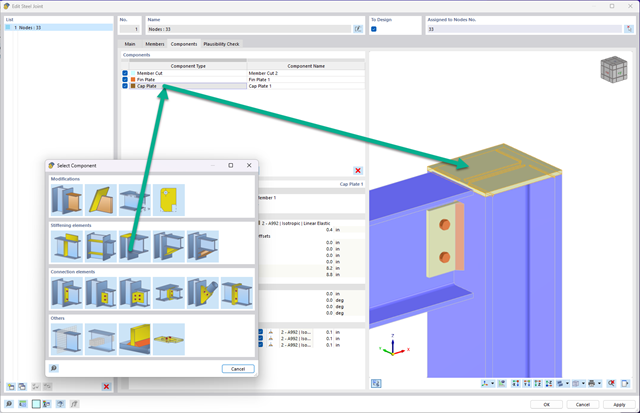
You can now insert a cap plate in steel joints with only a few clicks. You can enter the data using the known definition types "Offsets" or "Dimensions and Position". By specifying a reference member and the cutting plane, it is also possible to omit the Member Section component.
This component allows you to easily model cap plates on column ends, for example.
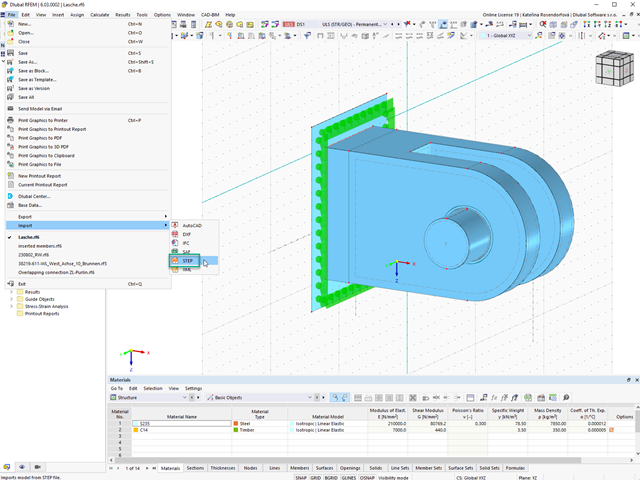
You can import STEP files into RFEM 6. The data is directly converted into the native RFEM model data.
The STEP format represents a standard interface initiated by ISO (ISO 10303). In the geometry description, all shapes relevant for RFEM (line, surface, and solid models) can be integrated by the CAD data models.
Note: This format is not to be confused with DSTV interfaces, which also use the file extension *.stp.
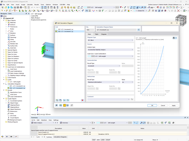
Do you want to create calculation diagrams? With RFEM and RSTAB, this works globally and without any problems. Create and organize your calculation diagrams directly in the Navigator - Data or via the menu Insert → Calculation Diagrams.
Use calculation diagrams to record and display a relation between the various calculation results.
It is also possible to superimpose similar diagrams.
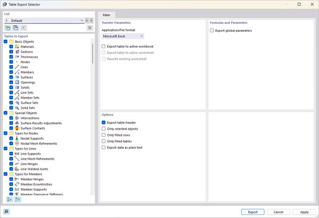
Did you know? You can export all RFEM/RSTAB tables with the results individually or all at once directly into an Excel table or as a CSV file. There are several options available to you:
- With table headers
- Selected objects only
- Filled rows only
- Only filled tables
- Export data as plain text
This way, the program allows you to control and clearly manage the exported data. You can export the stored formulas directly in the table or as a separate table, as in the case of the used parameters.

Your data are always documented in a multilingual printout report. You can adjust the content at any time and save it as a template. You can also add graphics, texts, MathML formulas, and PDF documents to your report with just a few clicks.

Note that the definition of the effective lengths in the Aluminum Design add-on is an essential requirement for the stability analysis. For this, define the nodal supports and effective length factors in the input dialog box. Do you want to clearly document the nodal supports and the resulting segments with the associated effective length factors? To check the input data, it is best for you to use the graphic display in the RFEM/RSTAB work window. Thus, you can comprehend the design at any time with minimum effort.
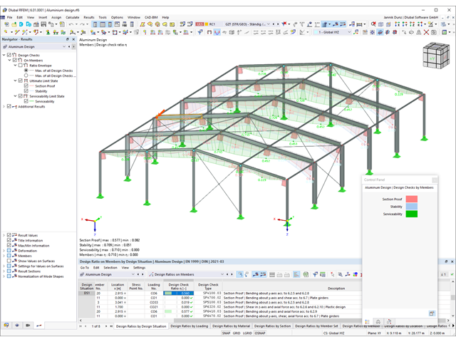
Was your design successful? Very good, now comes the relaxed part. Because the program gives you the performed design checks in a table. You can display all result details in detail here. The clearly presented design formulas ensure that you will be able to understand the results without any problems. There is no black-box effect with Dlubal Software.
The design checks are carried out at all governing locations of the members and displayed graphically as a result diagram. You can find more detailed graphics in the result output. This includes the stress distribution on the cross-section or the governing mode shape, for example.
All input and result data are part of the RFEM/RSTAB printout report. You can select the report contents and extent specifically for the individual design checks.

Enter and model a soil solid directly in RFEM. You can combine the soil material models with all common RFEM add-ons.
This allows you to easily analyze the entire models with a complete representation of the soil-structure interaction.
All parameters required for the calculation are automatically determined from the material data that you have entered. The program then generates the stress-strain curves for each FE element.

Did you know? You can enter the soil layers that you have obtained from the subsoil expertises done in the locations into the program in the form of soil samples. Assign the explored soil materials, including their material properties, to the layers.
For the definition of the samples, you can enter the data in tables as well as in the respective editing dialog box. Furthermore, you can also specify the groundwater level in the soil samples.

The soil solids that you want to analyze are summarized in soil massifs.
Use the soil samples as a basis for a definition of the respective soil massif. This way, the program allows for user-friendly generation of the massif, including the automatic determination of the layer interfaces from the sample data, as well as the groundwater level and the boundary surface supports.
Soil massifs provide you with the option to specify a target FE mesh size independently of the global setting for the rest of the structure. You can thus consider the various requirements of the building and soil in the entire model.
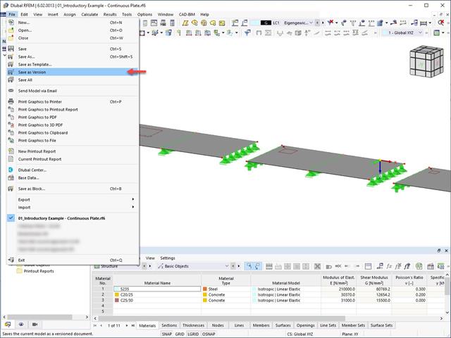
It is possible to save different model versions within a model by using the Save as Version function. In the Base Data of the model, the different model versions can be displayed in the History tab.

When defining the input data for the modal analysis load case, you can consider a load case whose stiffnesses represent the initial position for the modal analysis. How do you do that? As shown in the image, select the "Consider initial state from" option. Now, open the "Initial State Settings" dialog box and define the type Stiffness as the initial state. In this load case, as of which is the initial state taken into account, you can consider the stiffness of the structural system when the tension members fail. The purpose of all of this: The stiffness from this load case is considered in the modal analysis. Thus, you obtain a clearly flexible system.
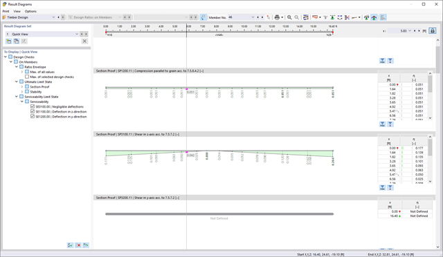
If your design is successful, the relaxed part of your work follows. Because the program does many processes for you. For example, the performed design checks are displayed in a table. It shows you all the result details. Due to the clearly presented design formulas, you will be able to understand the results without any problems. There is no "black box" effect here.
The design checks are carried out at all governing locations of the members and displayed graphically as a result diagram. Furthermore, detailed graphics, such as the stress distribution on a cross-section or the governing mode shape, are available for you in the result output.
All input and result data are part of the RFEM/RSTAB printout report. You can select the report contents and extent specifically for the individual design checks.
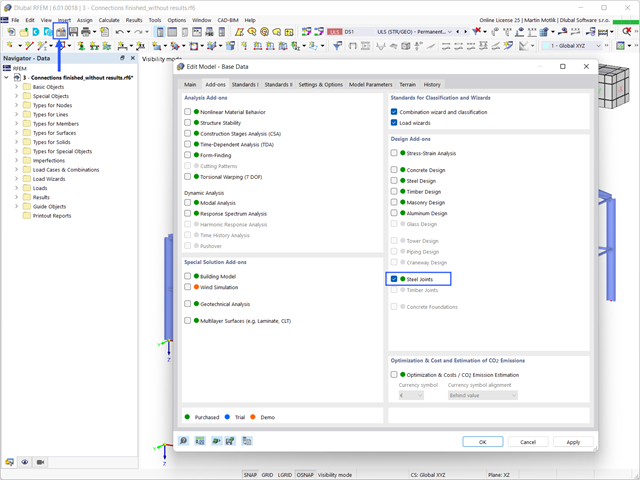
To design a Steel connection, you must have the Steel Joints Add-on enabled. The Add-ons in RFEM 6 are activated in the Add-ons tab of the Edit Model - Base Data window. If the Add-on is active, it is displayed in the navigator.
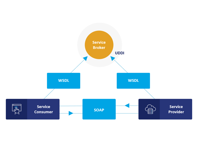
Communication is the key to success. This also applies to a client-server relation. WebService and API provides you with an XML based information exchange system for direct client-server communication. Programs, objects, messages, or documents can be integrated into these systems. For example, a web service protocol of the HTTP type runs for the client-server communication when you are looking for something in the Internet using a search engine.
Now back to Dlubal Software. In our case, the client is your programming environment (.NET, Python, JavaScript) and the service provider is RFEM 6. Client-server communication allows you to send requests to and receive feedback from RFEM, RSTAB, or RSECTION.
What is the difference between WebService and an API?
- WebService is a collection of open source protocols and standards used to exchange data between systems and applications. In contrast, an application programming interface (API), is a software interface through which two applications can interact without a user being involved.
- Thus, all web services are APIs, but not all APIs are web services.
What are the advantages of the WebService technology?
You can communicate more quickly within and between organizations.A service can be independent of other services.Webservice allows you to use your application to make your message or feature available to the rest of the world.Webservice helps you to exchange data between different applications and platforms Several applications can communicate, exchange data, and share services with each other. SOAP ensures that programs created on different platforms and based on different programming languages can exchange data securely.
Communication between the web service client and server is optionally encrypted via the https protocol. To do this, you can install an SSL certificate with the corresponding private key in the settings.
.jpg?mw=640&hash=26a7c7d3eca4bc6f129e08b373eac4f2314109ba)
Take your structural design one step further. RFEM 6 and RSTAB 9 support now a new file format for structural design, Structural Analysis Format (SAF). For this, both programs allow for the import as well as the export. SAF is a file format based on MS Excel, intended to facilitate the exchange of structural analysis models between different software applications.
You can now work even more efficiently with the Data Navigator. Its clear structure makes it easy to use. The navigator contains assignable types for objects as well as a hyperlink function that allows you to quickly jump to the assigned elements of an object.
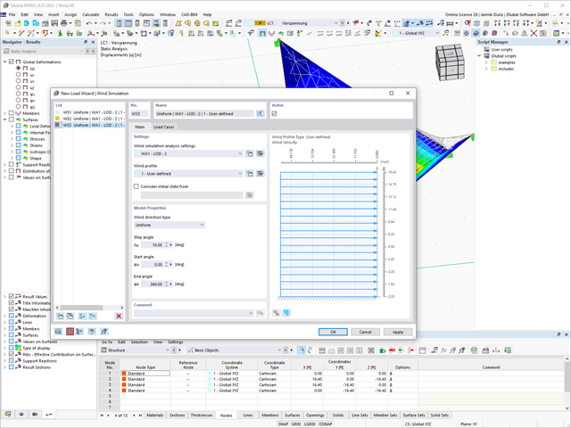
To model structures in RWIND Basic, you find a special application in RFEM and RSTAB. Here, you define the wind directions to be analyzed by means of related angular positions about the vertical model axis. At the same time, you define the elevation-dependent wind profile on the basis of a wind standard. In addition to these specifications, you can use the stored calculation parameters to determine your own load cases for a stationary calculation per each angular position.
As an alternative, you can also use the RWIND Basic program manually, without the interface application in RFEM or RSTAB. In this case, RWIND Basic models the structures and terrain environment directly from the imported VTP, STL, OBJ, and IFC files. You can define the height-dependent wind load and other fluid-mechanical data directly in RWIND Basic.
.jpg?mw=640&hash=81d73d5501397b910013fb09e66e758eaa32bd62)
There are also improvements in the data exchange to make your work process easier. In addition to the import of IFC 2x3 (Coordination View & Structural Analysis View), the import and export of IFC 4 (Reference View & Structural Analysis View) is now supported.